

The research question: which clock is volatility using?
On a quiet Sunday, the words gold volatility can seem to denote one observable object. In practice, they describe several different measurements taken from different instruments over different intervals. A five-minute XAU/USD range, a daily sequence of gold futures returns, an option-derived 30-day expectation and the twice-daily London benchmark are not interchangeable observations. The research question is therefore precise: when these measures disagree, is the disagreement new information about gold, or merely the consequence of different clocks? The distinction matters because traders often react to a number before asking what generated it. A number can be accurate inside its own definition yet misleading when inserted into an unrelated decision.
The Cboe Gold ETF Volatility Index, GVZ, is calculated from options on the SPDR Gold Shares exchange-traded fund, rather than from an uninterrupted spot-gold tape. Cboe's published methodology describes a forward-looking, constant-30-day measure inferred from option quotations [1]. That is an estimate embedded in option prices, not a report that gold will rise, fall or travel a specified distance during the next session. Even the choice of underlying matters: GLD options introduce an equity-market trading calendar and their own order-book characteristics. Calling GVZ the volatility of every gold instrument erases those differences before analysis begins.
CME Group explains a second essential distinction: implied volatility comes from options prices, whereas realized volatility summarizes movement that already occurred [2]. Neither is a direct measurement of fear inside a trader, and their numerical values need not coincide. The options market can price uncertainty, asymmetry and the willingness to pay for protection; subsequent realized moves can be calmer or more violent. That gap does not, by itself, prove options were irrational or that a behavioral signal anticipated anything. It first raises questions about contracts, expiry, return sampling, annualization and the market conditions represented by each dataset.
One metal, several markets and timestamps
The London Bullion Market Association describes the LBMA Gold Price as an auction benchmark set twice each London business day, at 10:30 and 15:00 local time, in US dollars per troy ounce [3]. Those fixing times are not a continuous intraday time series. A researcher who computes daily changes from benchmark observations is sampling two discrete reference points, while a person watching a continuous XAU/USD feed may see reversals and widening spreads between them. The benchmark can be appropriate for valuation and contracts without being a faithful proxy for every executable quote a retail trader could have obtained throughout that day.
Gold futures add another clock: a futures price embeds contract specifications, delivery timing and financing economics. The nearby contract is not identical to a London spot benchmark, even if their prices are economically related. Our earlier analysis of gold futures contango distinguishes a basis relationship from a directional prediction. That distinction becomes more important when comparing option-implied volatility derived from a listed futures or ETF market with spot-range statistics. The appropriate question is not which quote is the real gold price in isolation, but which claim each quoted series can support under a documented measurement protocol.
Calendar definitions create another layer. A market data vendor might label a bar by UTC while an exchange defines its session in Central Time and a Dubai-based desk reviews it on the Asia/Dubai date. Daylight-saving adjustments and maintenance windows can push the same execution into a different calendar bucket. An apparent change in the next day's volatility can therefore be a clock-alignment artifact. Researchers must publish time zone, contract identity, trading-session boundaries, whether missing bars are forward-filled and the convention for choosing a daily close. Without these, a result can be numerically reproducible inside one platform while remaining economically uninterpretable outside it.
Why the most dramatic number is often the least transferable
Consider a hypothetical announcement minute in which the quoted XAU/USD midpoint jumps sharply while market depth collapses. A one-minute realized-range calculation will register a large change; a 30-day option-based index may barely adjust if investors interpret the disturbance as short-lived and already anticipated. Conversely, options can reprice before a release while the spot range remains compressed. These are not contradictory descriptions. The measures answer different questions: what moved during one observation window, versus what options markets currently embed about future variability. A responsible narrative records the event window and the instrument before attaching a causal explanation.
Liquidity complicates that reading further. The difference between executable bid and ask, market depth, transaction costs and the price midpoint is not just a technical footnote. As discussed in a tight spread analysis, the visible spread alone may conceal the cost of filling an order when quoted size is small or disappearing. A spike calculated from last-traded prices may incorporate prints unavailable at the intended order size, while a midpoint-based statistic may understate immediate trading costs. This is especially important when researchers try to connect physiological observations, chart volatility and trading results in one timeline.
Sampling choices matter even for an uncontroversial historical series. A daily-close standard deviation suppresses intraday reversals by design; an intraday realized measure can amplify market-microstructure noise if sampled too frequently. A range-based estimator emphasizes highs and lows, which may be affected by quote quality and data cleaning. An options-implied statistic is model- and market-dependent and usually requires an explicit horizon. Comparing these measurements without normalization can turn a mechanical difference into an invented story about regime change. The observation is a variance in measurement; the hypothesis is that the underlying market state changed. They are not the same claim.
An evidence-first protocol for the NSI research lab
An NSI-style observational study should start by naming one primary outcome and one primary horizon before opening a chart. For example, it might ask whether a predefined physiological feature is associated with a change in a particular gold-market variability statistic over the following hour. It must identify the source instrument, session calendar, quote cleaning and how the market statistic is computed. Additional windows can be reported as sensitivity analyses, not quietly substituted after researchers see which one looks strongest. The NSI concept remains a proposed research framework; no independently validated ability to predict gold prices or diagnose a person's condition follows from such a design.
Next, the study should synchronize the relevant timestamps, separate in-sample model selection from prospective evaluation and preserve the decisions made before data collection. If a signal appears strongest at fifteen minutes but not at five, sixty or three hundred minutes, that pattern is a finding to investigate, not a license to declare fifteen minutes the system's true frequency. Multiple horizons multiply the opportunities for chance findings. Reporting the full grid and the out-of-sample behavior is more informative than presenting only the attractive cell. London gold clearing and benchmark conventions should be described separately when they form part of the reference dataset.
A final analysis should distinguish forecast calibration from economic usefulness. A model could anticipate that realized volatility will be higher on average while providing little help with execution price, direction or position sizing. Likewise, an accurate option-derived volatility index can describe aggregate expectations without dictating a profitable trade. A meaningful research conclusion states the interval, population, instruments, uncertainty estimates and failure cases, then specifies what independent replication would need to demonstrate. The practical lesson is narrower and stronger than a headline: first align the clocks, then compare the measurements, and only afterward test a causal or predictive claim.
Scientific bibliography & sources
- [1] Cboe Global Markets, Volatility Index Methodology: Selected Broad-Based Index, Equity and ETF Volatility Indices, including GVZ (2026). https://cdn.cboe.com/api/global/us_indices/governance/Volatility_Index_Methodology_Selected_Broad_Based_Index_Equity_and_ETF_Volatility_Indices.pdf
- [2] CME Group, Understanding the CVOL Index: Implied Versus Realized Volatility. https://www.cmegroup.com/education/courses/introduction-to-cvol/understanding-the-cvol-index
- [3] London Bullion Market Association, About LBMA Daily Auction Prices. https://www.lbma.org.uk/prices-and-data/about-lbma-daily-auction-prices
Research note
NSI is a proposed research framework, not an independently validated medical or financial prediction system. This article is research and education, not individualized medical or investment advice. Market observations are timestamped historical context, not live prices.
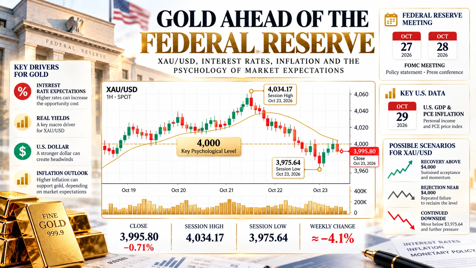 Market
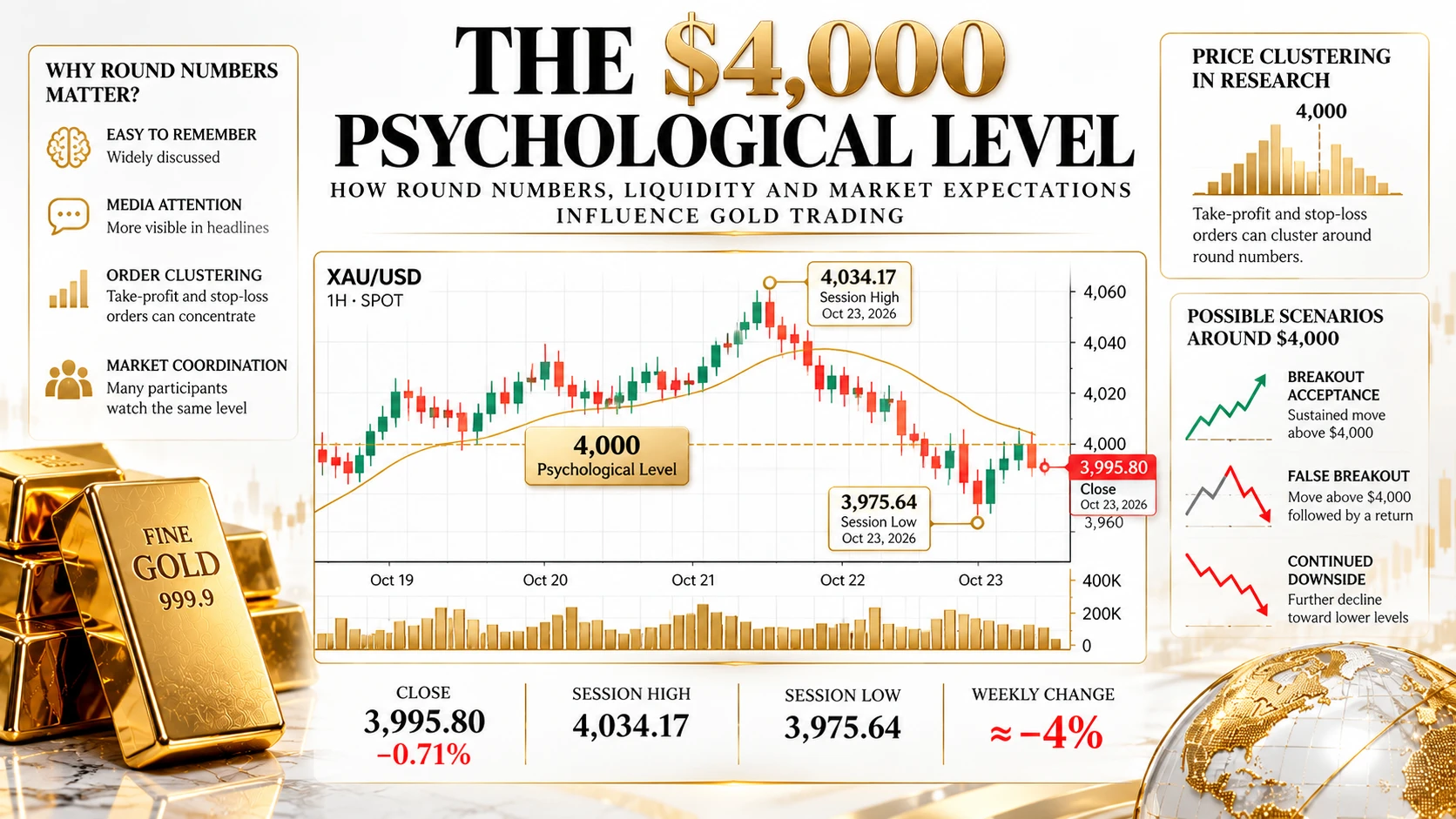 Market
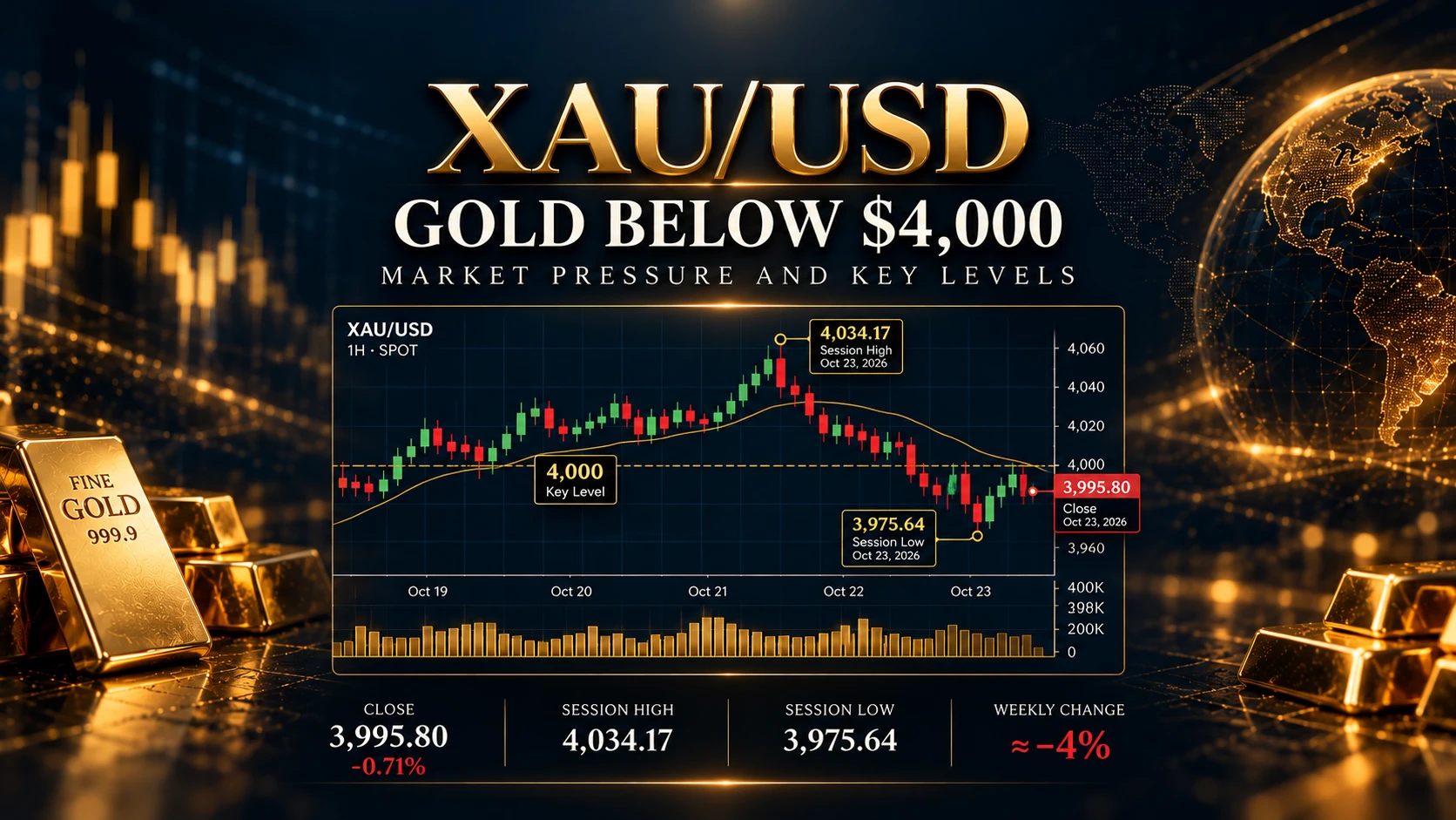 Market